Monte Carlo Tree Search
- Keep descending until you explore a new leaf node. Walk down from the root, at each node picking the child whose PUCT score is highest.
- Evaluate the leaf node's policy and value.
- Walk the leaf's value back up to the root (increment each intermediate node's visit count and fold the leaf value into its running average).
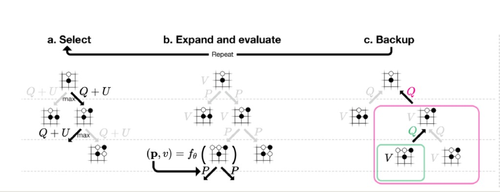
Figure 2 from Silver et al., 2017.
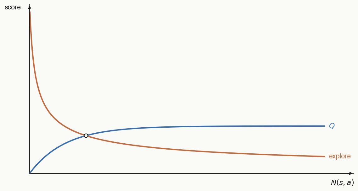
Unvisited children have a tiny denominator (just ), so their explore term is huge — they get tried first. Each subsequent visit makes less-visited siblings relatively more attractive and the move under consideration less attractive: the denominator grows linearly while in the numerator grows only as a square root.
The prior sets the order: high-prior moves get the biggest bonus and are tried first, low-prior moves later.
Thus the MCTS-derived is leaned on more to determine the value of a node when you have visited it more.
- Neural network: — the policy prior, written into a node once, when that node is first expanded.
- MCTS node: , , — all running statistics of the search itself.
An online running mean of the leaf values reached by simulations that passed through this edge.
What the neural network does
To guide and prune the MCTS search.
- Input: the current board state.
- Outputs: a policy — a probability distribution over the legal moves — and a value — the probability the current player will win.
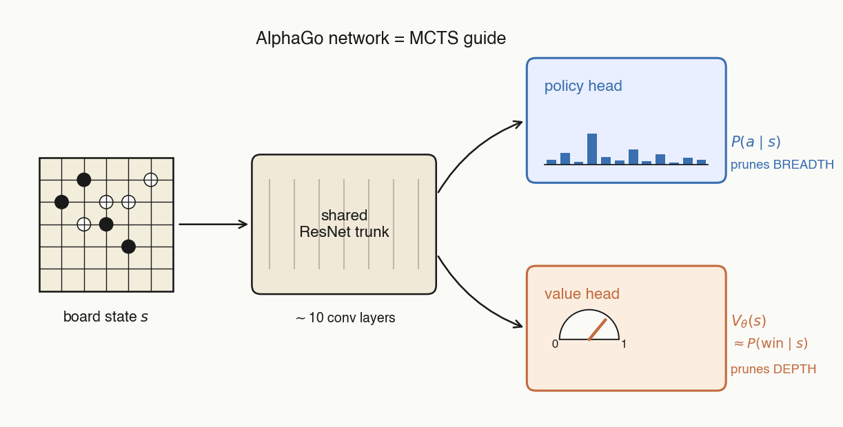
- Policy head prunes breadth. goes into PUCT's exploration term, so MCTS spends ~no visits on obviously bad moves.
- Value head prunes depth. When you visit a new node, you just take the value head's prediction of winning for granted and percolate it up the MCTS tree.
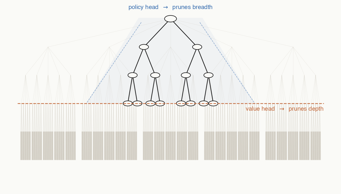
- To do argmax over the values of potential next moves, you'd have to run a forward pass of the value network up to 361 times — whereas one forward pass of the policy gives you the distribution over all moves at once.
- You can't easily turn MCTS into a single scalar, and the whole point of training is to distill the MCTS search into the model.
Most Go fighting is local: captures, ladders, life-and-death problems. Convolutional receptive fields encode "what's near this stone matters most," and a useful local pattern is learned once and reused everywhere on the board.
Eric addendum: "With larger-scale data + compute, transformers can learn these biases from scratch, but it didn't emerge at the scale of experiments I was trying."
Go is a perfect-information game, so the current board encodes all the relevant information — there's a Nash-equilibrium strategy that depends only on .
In hidden-information games like poker or Diplomacy that breaks: the value of your hand depends on the opponent's earlier bluffs, alliances, betting patterns. Now you need an architecture that carries state across time (RNN, or Transformer over a history of states), not just one that attends over space.
Self-play
- For the policy head: the final MCTS visit distribution at that move.
- For the value head: who won the game, projected (with appropriate sign flips for self-play) back through every move.
Conceptually:
- Make the value head predict who actually won.
- Make the policy head predict the MCTS visit distribution at that state.
Mathematically, summed over states visited in self-play:
Alternate RL approaches
Two evenly-matched policies play 100 games of ~300 moves each. By chance, maybe one game is won by a genuinely better move; the other ~50 wins are statistical noise. Imitating winners gives you one useful gradient buried inside ~30,000 neutral move labels — drowned out.
MCTS distillation has no credit-assignment problem. Instead of "this game was won, copy these moves," it says: at every state you visited, here is a strictly better move than the one you played. Every move becomes a dense per-state supervision target — like DAgger interventions in imitation learning.
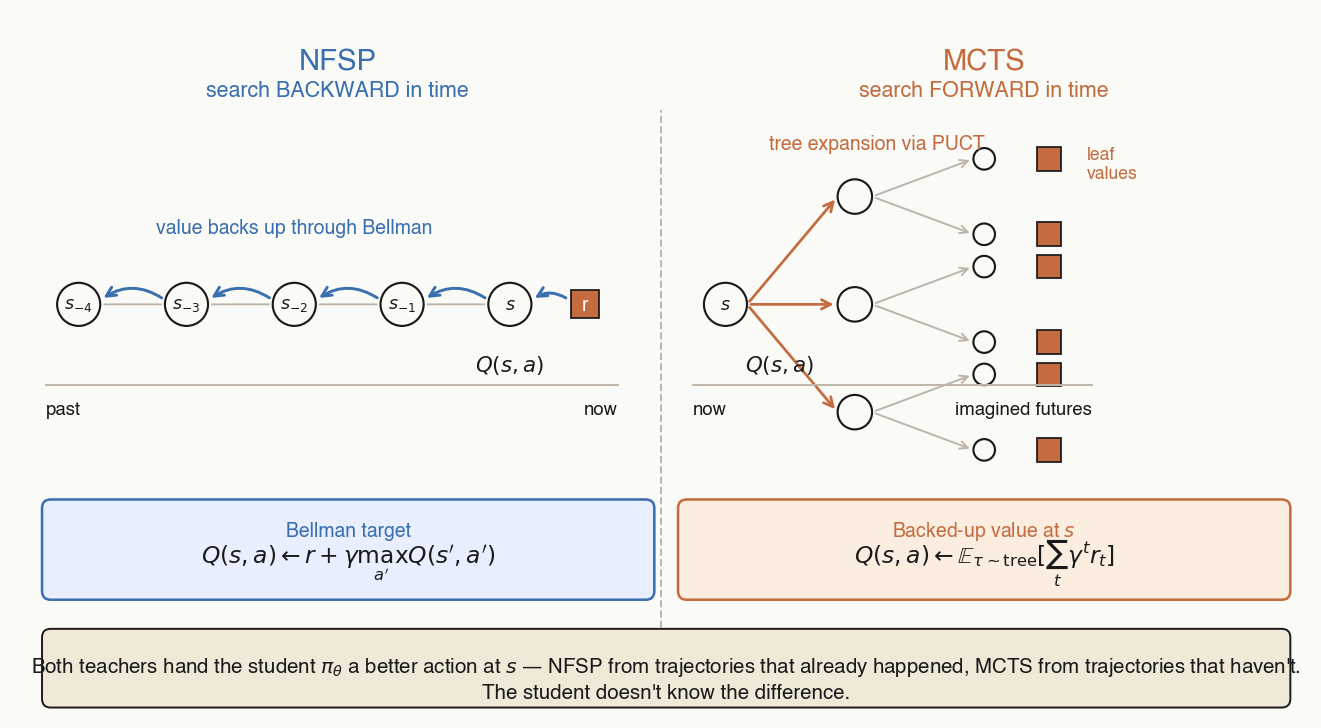
- NFSP — search backward in time. Bellman/TD backup over trajectories that already happened.
- MCTS — search forward in time. UCT tree expansion over trajectories that haven't happened yet.
Why doesn't MCTS work for LLMs
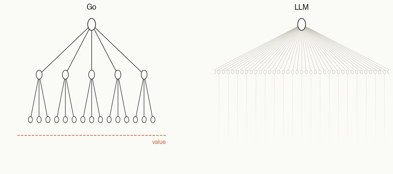
- Unbounded breadth. The number of legal actions from a given state (i.e. what further thoughts one could have started from a partial reasoning trace) is essentially unbounded — whereas for Go, there's at most 361 legal next moves.
- Harder to prune depth. Much harder to train a value model to anticipate whether a partial coding or thinking trajectory will result in success than whether a given board state is favorable to you.